defcompute_cost(x, y, w, b): """ Computes the cost function for linear regression. Args: x (nd_array): Data, m examples y (nd_array): target values w,b (scalar): model parameters Returns total_cost (float): The cost of using w,b as the parameters for linear regression to fit the data points in x and y """ # number of training examples m = x.shape[0] #using numpy cost_sum = 0 for i inrange(m): f_wb = w * x[i] + b cost = (f_wb - y[i]) ** 2 cost_sum = cost_sum + cost total_cost = (1 / (2 * m)) * cost_sum
defcompute_gradient(x, y, w, b): """ Computes the gradient for linear regression Args: x (nd_array): Data, m examples y (nd_array): target values w,b (scalar): model parameters Returns dj_dw (scalar): The gradient of the cost w.r.t. the parameters w dj_db (scalar): The gradient of the cost w.r.t. the parameter b """ # Number of training examples m = x.shape[0] dj_dw = 0 dj_db = 0 for i inrange(m): f_wb = w * x[i] + b dj_dw_i = (f_wb - y[i]) * x[i] dj_db_i = f_wb - y[i] dj_db += dj_db_i dj_dw += dj_dw_i dj_dw = dj_dw / m dj_db = dj_db / m return dj_dw, dj_db
defgradient_descent(x, y, w_0, b_0, alpha, num_iters): """ Performs gradient descent to fit w,b. Updates w,b by taking num_iters gradient steps with learning rate alpha Args: x (nd_array): Data, m examples y (nd_array): target values w_0,b_0 (scalar): initial values of model parameters alpha (float): Learning rate num_iters (int): number of iterations to run gradient descent Returns: w (scalar): Updated value of parameter after running gradient descent b (scalar): Updated value of parameter after running gradient descent J_history (List): History of cost values p_history (list): History of parameters [w,b] """ w = copy.deepcopy(w_0) # avoid modifying global w_0 # An array to store cost J and w's at each iteration primarily for graphing later J_history = [] p_history = [] b = b_0 w = w_0 for i inrange(num_iters): # Calculate the gradient and update the parameters using gradient_function dj_dw, dj_db = compute_gradient(x, y, w , b)
# Update Parameters b = b - alpha * dj_db w = w - alpha * dj_dw
# Save cost J at each iteration if i < 100000: # prevent resource exhaustion J_history.append(compute_cost(x, y, w , b)) p_history.append([w,b]) # Print cost every at intervals 10 times or as many iterations if < 10 if (i % math.ceil(num_iters/10)) == 0: print(f"Iteration {i:4}: Cost {J_history[-1]:0.2e} ", f"dj_dw: {dj_dw: 0.3e}, dj_db: {dj_db: 0.3e} ", f"w: {w: 0.3e}, b:{b: 0.5e}") return w, b, J_history, p_history #return w,b and J,p history for graphing
Multiple Variables Linear Regression
Model
The model’s prediction with multiple variables is given by the linear model:
or in vector notation:
where $\cdot$ is a vector dot product
1
2
3
x = np.array([1,2,3])
y = np.array([4,5,6])
f = np.dot(w,x) + b #we can use numpy dot to calculate
Examples are stored in a NumPy matrix . Each row of the matrix represents one example. When you have $m$ training examples, and there are $n$ features, $\mathbf{X}$ is a matrix with dimensions ($m$, $n$) (m rows, n columns).
notation:
$\mathbf{x}^{(i)}$ is vector containing example i. $\mathbf{x}^{(i)}$ $ = (x^{(i)}_0, x^{(i)}_1, \cdots,x^{(i)}_{n-1})$
$x^{(i)}_j$ is element j in example i . The superscript in parenthesis indicates the example number while the subscript represents an element.
$\mathbf{w}$ is a vector with $n$ elements.
Each element contains the parameter associated with one feature.
notionally, we draw this as a column vector
$b$ is a scalar parameter.
Cost Function
The equation for the cost function with multiple variables $J(\mathbf{w},b)$ is:
where:
Gradient Descent
Gradient descent for multiple variables:
for j = 0..n-1, where, n is the number of features, parameters $w_j$, $b$, are updated simultaneously and where
m is the number of training examples in the data set
$f_{\mathbf{w},b}(\mathbf{x}^{(i)})$ is the model’s prediction, while $y^{(i)}$ is the target value
For a logistic regression model , $f_{\mathbf{w},b}(\mathbf{x}^{(i)}) = \mathbf{w} \cdot \mathbf{x}^{(i)} + b$
Feature Scaling
Mean Normalization
Z-Score Normalization
where $j$ selects a feature or a column in the X matrix. $\mu_j$ is the mean of all the values for feature (j) and $\sigma_j$ is the standard deviation of feature (j).
Code in Python
1
2
3
4
5
6
7
8
9
10
11
12
13
14
15
16
17
defcompute_cost(X, y, w, b): """ Args: X (matrix (m,n)): Data, m examples with n features y (nd_array (m,)) : target values w (nd_array (n,)) : model parameters b (scalar) : model parameter Returns: cost (scalar): cost """ m = X.shape[0] cost = 0.0 for i inrange(m): f_wb_i = np.dot(X[i], w) + b cost = cost + (f_wb_i - y[i])**2 cost = cost / (2 * m) return cost
defcompute_gradient(X, y, w, b): """ Args: X (matrix (m,n)): Data, m examples with n features y (nd_array (m,)) : target values w (nd_array (n,)) : model parameters b (scalar) : model parameter Returns: dj_dw (nd_array (n,)): The gradient of the cost w.r.t. the parameters w. dj_db (scalar): The gradient of the cost w.r.t. the parameter b. """ m,n = X.shape #(number of examples, number of features) dj_dw = np.zeros((n,)) #create a new array dj_db = 0.0
for i inrange(m): err = (np.dot(X[i], w) + b) - y[i] for j inrange(n): dj_dw[j] = dj_dw[j] + err * X[i, j] dj_db = dj_db + err dj_dw = dj_dw / m dj_db = dj_db / m return dj_db, dj_dw
defgradient_descent(X, y, w_in, b_in, alpha, num_iters): """ Args: X (matrix (m,n)) : Data, m examples with n features y (nd_array (m,)) : target values w_in (nd_array (n,)) : initial model parameters b_in (scalar) : initial model parameter alpha (float) : Learning rate num_iters (int) : number of iterations to run gradient descent Returns: w (nd_array (n,)) : Updated values of parameters b (scalar) : Updated value of parameter """ # An array to store cost J and w's at each iteration primarily for graphing later J_history = [] w = copy.deepcopy(w_in) #avoid modifying global w within function b = b_in for i inrange(num_iters): # Calculate the gradient and update the parameters dj_db,dj_dw = compute_gradient(X, y, w, b)
# Update Parameters using w, b, alpha and gradient w = w - alpha * dj_dw b = b - alpha * dj_db # Save cost J at each iteration if i<100000: # prevent resource exhaustion J_history.append(compute_cost(X, y, w, b))
# Print cost every at intervals 10 times or as many iterations if < 10 if (i % math.ceil(num_iters / 10)) == 0: print(f"Iteration {i:4d}: Cost {J_history[-1]:8.2f}") return w, b, J_history #return final w,b and J history
1
2
3
4
5
6
7
8
9
10
11
12
13
14
15
import numpy as np defzscore_normalize_features(X): """ computes X, zcore normalized by column Args: X (nd_array): Shape (m,n) input data, m examples, n features Returns: X_norm (nd_array): Shape (m,n) input normalized by column mu (nd_array): Shape (n,) mean of each feature sigma (nd_array): Shape (n,) standard deviation of each feature """ mu= np.mean(X, axis=0) sigma = np.std(X, axis=0) X_norm = (X - mu) / sigma return (X_norm, mu, sigma)
Logistic Regression
Sigmoid Function
A logistic regression model applies the sigmoid to the linear regression model as shown below:
where $g(z)$ is shown above.
Therefore, to get a final prediction ($y=0$ or $y=1$) from the logistic regression model, we can use the following
if $f_{\mathbf{w},b}(x) \ge 0.5$, predict $y=1$
if $f_{\mathbf{w},b}(x) < 0.5$, predict $y=0$
$\mathbf{w} \cdot \mathbf{x} + b = 0$ is the decision boundary. It can be linear or non-linear, depending on what kinds of features you are using. If you use all linear features, it will be a line. Or if you have $x^2,x^3…$, it may be a complex curve line.
Loss Function
$loss(f_{\mathbf{w},b}(\mathbf{x}^{(i)}), y^{(i)})$ is the cost for a single data point, which is:
$f_{\mathbf{w},b}(\mathbf{x}^{(i)})$ is the model’s prediction, while $y^{(i)}$ is the target value.
$f_{\mathbf{w},b}(\mathbf{x}^{(i)}) = g(\mathbf{w} \cdot\mathbf{x}^{(i)}+b)$ where function $g$ is the sigmoid function.
it can also be written as:
Cost Function
Logistic Gradient Descent
Where each iteration performs simultaneous updates on $w_j$ for all $j$, where
m is the number of training examples in the data set
$f_{\mathbf{w},b}(x^{(i)})$ is the model’s prediction, while $y^{(i)}$ is the target
For a logistic regression model $z = \mathbf{w} \cdot \mathbf{x} + b$ $f_{\mathbf{w},b}(x) = g(z)$ where $g(z)$ is the sigmoid function: $g(z) = \frac{1}{1+e^{-z}}$
Overfitting And Regularization
To addressing overfit problem ,we can add a regularization term to the cost function.
In linear regression, It will be:
In logistic regression, it will be:
And we can calculate derivative term when performing gradient descent as following:
Code in Python
1
2
3
4
5
6
7
8
9
10
11
import numpy as np defsigmoid(z): """ Compute the sigmoid of z Args: z (nd_array): A scalar, numpy array of any size. Returns: g (nd_array): sigmoid(z), with the same shape as z """ g = 1/(1+np.exp(-z)) return g
1
2
3
4
5
6
7
8
9
10
11
12
13
14
15
16
17
18
19
defcompute_cost_logistic(X, y, w, b): """ Computes cost Args: X (ndarray (m,n)): Data, m examples with n features y (ndarray (m,)) : target values w (ndarray (n,)) : model parameters b (scalar) : model parameter Returns: cost (scalar): cost """ m = X.shape[0] total_cost = 0 f_w = sigmoid(np.dot(X, w) + b) for i inrange(m): temp_cost = -y[i]*np.log(f_w[i]) - (1-y[i])*np.log(1-f_w[i]) total_cost += temp_cost total_cost = total_cost / m return cost
defcompute_gradient_logistic(X, y, w, b): """ Computes the gradient for logistic regression Args: X (ndarray (m,n): Data, m examples with n features y (ndarray (m,)): target values w (ndarray (n,)): model parameters b (scalar) : model parameter Returns dj_dw (ndarray (n,)): The gradient of the cost w.r.t. the parameters w. dj_db (scalar) : The gradient of the cost w.r.t. the parameter b. """ m,n = X.shape dj_dw = np.zeros((n,)) dj_db = 0.
err = sigmoid(np.dot(X, w) + b) - y for j inrange(n): for i inrange(m): dj_dw[j] += err[i] * X[i,j] dj_dw = dj_dw / m dj_db = np.sum(err) / m return dj_db, dj_dw
Neual Network
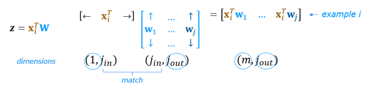
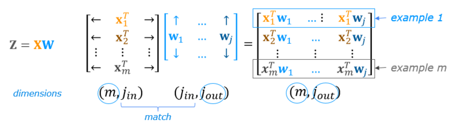
Matrix Multiply
$\mathcal{x_i}^T$ : a single example in training dataset
$\mathcal{W}$: the parameters matrix
$\mathcal{Z = XW +B}$
Neurons And Layers
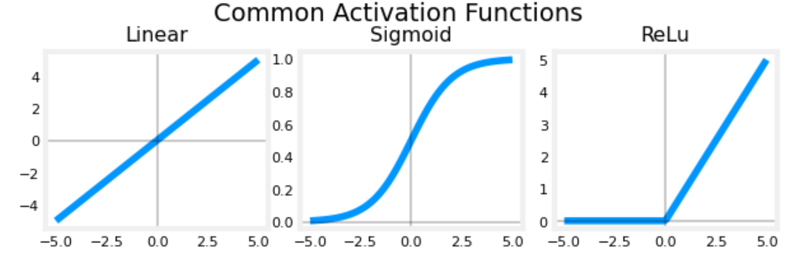
Neuron without activation - Regression/Linear Model
Each neuron performs once linear model as following:
suitable for $y \in (-\infty , + \infty)$
Neuron with Sigmoid activation
Each neuron performs once sigmoid function:
where
suitable for binary classification, $y = 0 ~~ or ~~ 1$
Neurons with ReLU activation (Rectified Linear Unit)
Each neuron performs once ReLU function:
where
suitable for $y \ge 0$
strongly recommended to apply ReLU activation in hidden neurons
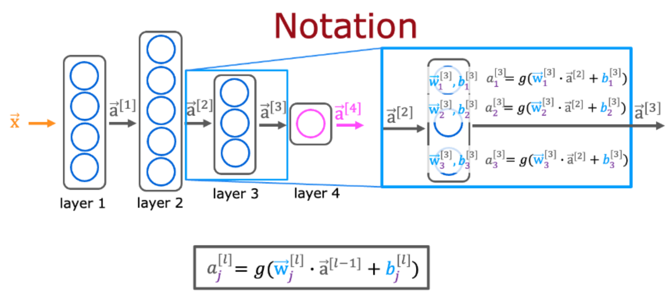
Mathematical form of Neural Network
$\vec{x}$: can be also written as $\vec{a}^{[0]}$, is the input of the neuron network
$a_j^{[l]}$: the $j^{th}$ neuron in the $l^{th}$ layer
$\vec{a}^{[l]}$: the output of the $l^{th}$ layer
$\vec{w}_j^{[l]}$: the parameter vector of the $j^{th}$ neuron in the $l^{th}$ layer
import numpy as np
import tensorflow as tf
from tensorflow.keras.layers import Dense, Input
from tensorflow.keras import Sequential
from tensorflow.keras.activations import linear, relu, sigmoid
from tensorflow.keras.losses import BinaryCrossentropy,MeanSquareError

#create a network:L1,L2,L3,...
#each layer has certain numbers of neurons:25,10,2,...
#dense layer is a common layer type
#activation function can be linear or sigmoid or relu
model = Sequential(
    [
tf.keras.Input(shape=(2,))
tf.keras.layers.Dense(units=25,activation="sigmoid",name="L1"),
tf.keras.layers.Dense(units=10,activation="sigmoid",name="L2"),
tf.keras.layers.Dense(units=1,activation="sigmoid",name="L3"),
        ...
    ]
)

X = np.array([[4,5],
              [1,8],
              [6,8],
              [6,6],
              [7,1],
              [6,5]],
             dtype=np.float32)
Y = np.array([[0],
              [0],
              [0],
              [1],
              [1],
              [1]],
              dtype=np.float32)
# input X,Y must be 2-D matrix

#create a "Normalization Layer" to get X normalized.
norm_l = tf.keras.layers.Normalization(axis=-1)
norm_l.adapt(X)# learns mean, variance of dataset
Xn = norm_l(X)

print(L1.get_weights())#return a numpy array
#>>>[array([[0.54]], dtype=float32), array([0.], dtype=float32)]

w,b = L1.get_weights()
print(w,b) #>>>[[0.54]] [0.]
print(w.shape,b.shape)#>>>(1, 1) (1,)
# w is a 2D matrix, b is a vector

set_w = np.array([[2]]) # w must be 2D matrix
set_b = np.array([-4.5])
L1.set_weights([set_w, set_b])#set weights manually


model.summary()
'''
shows the layers and number of parameters in the model.
Model: "sequential_3"
┏━━━━━━━━━━━━━━━━━━━┳━━━━━━━━━━━━━━━━━━━━━━━━┳━━━━━━━━━━━━━┓
┃ Layer (type)    ┃ Output Shape         ┃    Param # ┃
┡━━━━━━━━━━━━━━━━━━━╇━━━━━━━━━━━━━━━━━━━━━━━━╇━━━━━━━━━━━━━┩
│ L1 (Dense)      │ (None, 25)           │         75 │
└─────────────────┴──────────────────────┴────────────┘
 Total params: 75 (300.00 B)
 Trainable params: 75 (300.00 B)
 Non-trainable params: 0 (0.00 B)
'''

# loss function can be BinaryCrossentropy or MeanSquareError
# 即二元交叉熵or均方误差
model.compile(
	loss = tf.keras.losses.BinaryCrossentropy(),
    optimizer = tf.keras.optimizers.Adam(learning_rate=0.01),
	) # generate the model

model.fit(
    Xn,Y
    epochs=100,
	) # run gradient descent to fit the model

model.predict(new_X)
a1=L1(Xn)
print(a1)
'''
>>>tf.Tensor(
[[0.5  0.5  0.5 ... ]
 [0.45 0.35 0.55 ...]
 [0.41 0.23 0.59 ...]
 [0.36 0.14 0.63 ...]
 [0.32 0.08 0.68 ...]
 [0.28 0.05 0.71 ...]], shape=(6, 25), dtype=float32)

 output is a tensor type data
 each row represent $\vec{a}^{[1]}_j$
'''
Multiclass Classification
Softmax Function
The softmax function can be written:
The output $\mathbf{a}$ is a vector of length N, so for softmax regression, you could also write:
Loss Function
The loss function associated with Softmax, called the sparse categorical cross-entropy loss(稀疏多分类交叉熵损失), is:
Cost Function
To write the cost function, we need to define an indicator function first:
Now the cost is:
Where $m$ is the number of examples, $N$ is the number of outputs.
import numpy as np import tensorflow as tf from tensorflow.keras.models import Sequential from tensorflow.keras.layers import Dense,Input from tensorflow.keras.activations import linear, relu, sigmoid from sklearn.datasets import make_blobs
''' generate cluster samples make_blobs() para: n_samples :sample numbers [int],default=100 n_features :dimension of samples [int],default=2 centers :labels of samples [int or vector((x,y),center of each label)] cluster_std:standard deviation [float or vector] random_state:random seeds ''' centers = [[-5, 2], [-2, -2], [1, 2], [5, -2]] X_train, y_train = make_blobs(n_samples=2000, centers=centers, cluster_std=1.0,random_state=30)
model = Sequential( [ tf.keras.Input(shape=(400,)), Dense(25, activation = 'relu'), Dense(15, activation = 'relu'), Dense(4, activation = 'linear') #<-- Attention! ] ) model.compile( loss=tf.keras.losses.SparseCategoricalCrossentropy(from_logits=True), #<-- Attention optimizer=tf.keras.optimizers.Adam(learning_rate=0.001), ) #write code in this way is highly recommended, to decrease float-computing error #output layer set as linear,and pass the results to loss function
'''The [.fit](https://www.tensorflow.org/api_docs/python/tf/keras/Model) method returns a variety of metrics including the loss. This is captured in the `history` variable above. This can be used to examine the loss in a plot as shown below.''' history = model.fit( X_train,y_train, epochs=10 ) ''' fig,ax = plt.subplots(1,1, figsize = (4,3)) ax.plot(history.history['loss'], label='loss') ax.set_ylim([0, 2]) ax.set_xlabel('Epoch') ax.set_ylabel('loss (cost)') ax.legend() ax.grid(True) plt.show()'''
p = model.predict(X_train)#The output predictions are not probabilities results = tf.nn.softmax(p).numpy()#the output should be be processed by a softmax. for i inrange(len(results)): print( f"{results[i]}, category: {np.argmax(results[i])}")
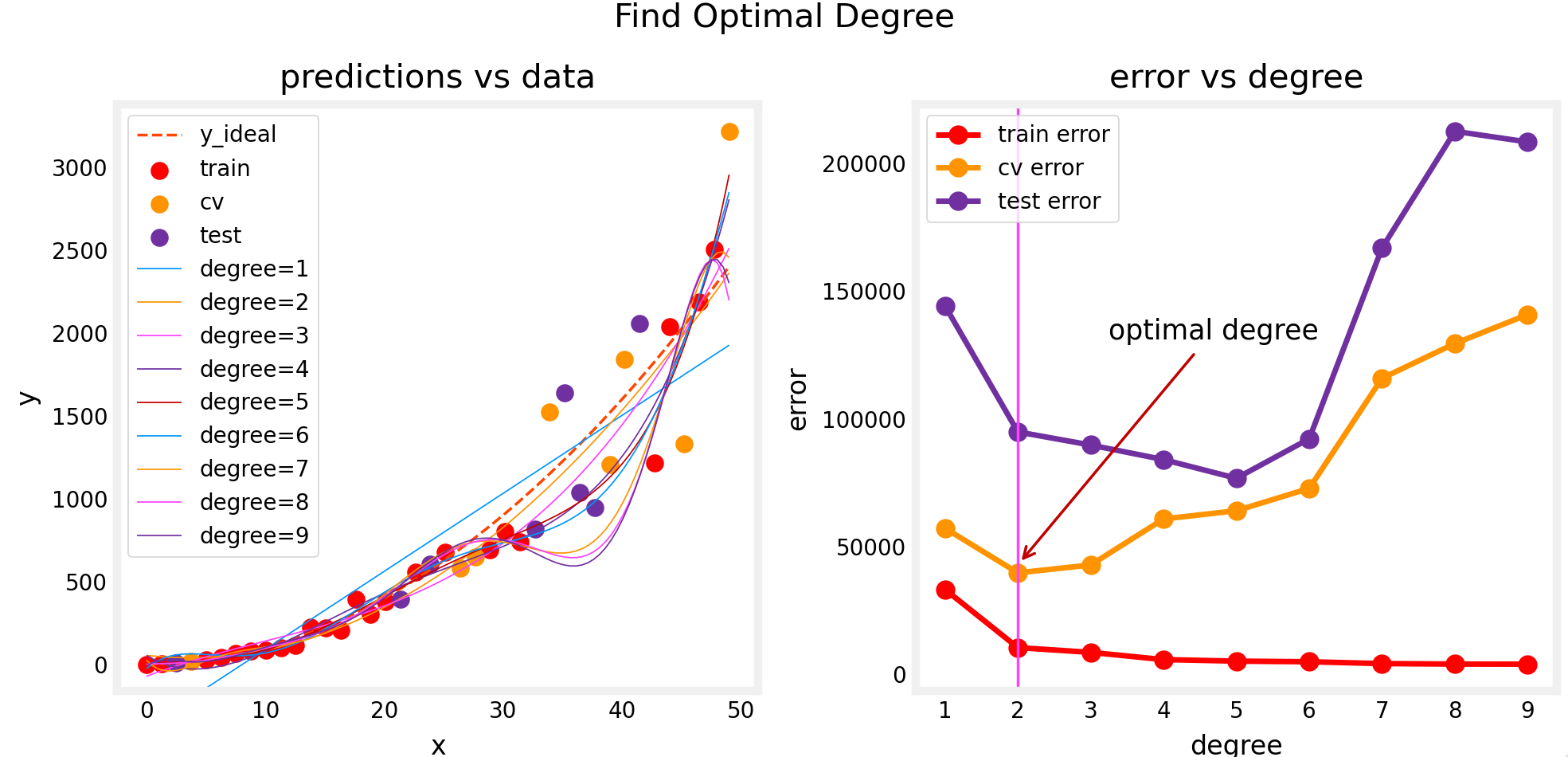
Choose the model which has the lowest cv error , even though it has a higher test error. ( To Avoid overfitting problem)
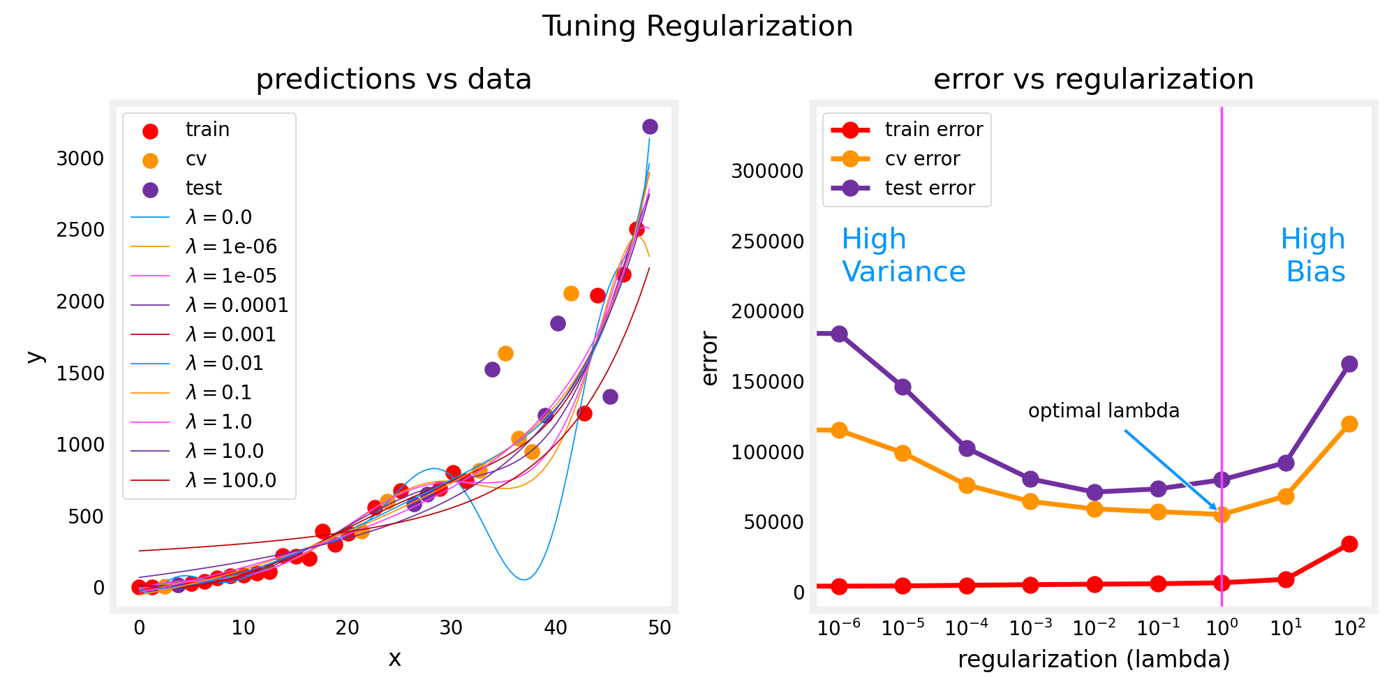
Tuning Regularization
Choose the model which has the lowest cv error
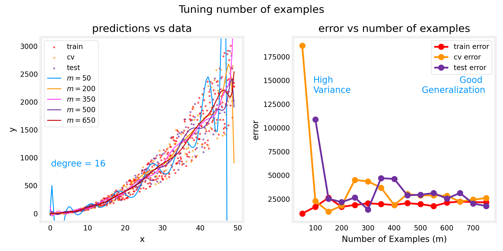
Increasing Training Set Size
When a model is overfitting (high variance), collecting additional data can improve performance.
Neural Network
simple model(less layers, less neurons) usually has a little higher classification error on training data but does better on cross-validation data than the more complex model.
apply regularization to moderate the impact of a more complex model!
(倾斜数据集) $y=1$ in presence of rare class we want to detect
Actual
Class
1
0
Predicted
1
True Positive
False Positive
Class
0
False Negative
True Negative
Precision:
Recall:
Trading off between precision and recall: we can define a F1 score to measure these two factors: A module which has a larger F1 score does better.
Decision Trees
One Hot Encoding
If a categorical feature can take on $k$ discrete (离散的) values, create $k$ binary features (0 or 1 valued).
Entropy
Note
$p_1$ stands for the fraction of label $y=1$ in a node
The log is calculated with base $2$
For implementation purposes, $0 \text{log}_2(0) = 0$. That is, if $p_1 = 0$ or $p_1 = 1$, set the entropy to 0
Information Gain
where
$H(p_1^\text{node})$ is entropy at the node
$H(p_1^\text{left})$ and $H(p_1^\text{right})$ are the entropies at the left and the right branches resulting from the split
$w^{\text{left}}$ and $w^{\text{right}}$ are the proportion of examples at the left and right branch respectively
Steps to Build a Decision Tree
Start with all examples at the root node
Calculate information gain for splitting on all possible features, and pick the one with the highest information gain
Split dataset according to the selected feature, and create left and right branches of the tree
Keep repeating splitting process until stopping criteria is met, which can be a maximum depth, examples in a node is below a threshold, information gain is very small…
Tree Ensemble
Bagged Decision Trees (Randomizing Samples)
Given training set of size m;
Use sampling with replacement(有放回随机抽样) to create a new training set of size m;
Train a tree in the new dataset;
Repeat step2 and step3 for n times, then we have a bag of trees which has n trees
Let all the trees voting for the result.
Random Forest (Randomizing Samples and Feature Choice)
At each node, when choosing a feature to use to split, if n features are available, pick a random subset of $k < n$ features and allow the algorithm to only choose from that subset of features
This can make trees much more different, improve computing speed and decrease overfitting.